Quickstart

To get started, you will need to install intake-esgf using pip:

python -m pip install intake-esgf

or conda-forge:

conda install -c conda-forge intake-esgf

Next you will need to import the ESGFCatalog and matplotlib for plotting later in the document.

from intake_esgf import ESGFCatalog
import matplotlib.pyplot as plt

Populate the Catalog¶

A catalog in intake-esgf initializes empty. This is because while intake-esm loads a large file-based database into memory, we are going to populate a catalog by searching one or many index nodes. The ESGFCatalog is configured by default to query a Globus-based index which has information about holdings at the Argonne Leadership Computing Facility (ALCF) only. We will demonstrate how this may be expanded to include other nodes later.

cat = ESGFCatalog()
print(cat)  # <-- nothing to see here yet

Perform a search() to populate the catalog.

To populate the catalog, perform a search using the traditional facets. If you are not familiar with these, we recommend you starting with our Beginner’s Guide to ESGF tutorial.

cat.search(
    experiment_id="historical",
    source_id="CanESM5",
    frequency="mon",
    variable_id=["gpp", "tas", "pr"],
)

cat

The search has populated the catalog where results are stored internally as a pandas dataframe, where the columns are the facets common to ESGF. Printing the catalog will display each column as well as a possibly-truncated list of unique values. We can use these to help narrow down our search. In this case, we neglected to mention a member_id (also known as a variant_label). So we can repeat our search with this additional facet. Note that searches are not cumulative and so we need to repeat the previous facets in this subsequent search. Also, while for the tutorial’s sake we repeat the search here, in your own analysis codes, you could simply edit your previous search.

cat.search(
    experiment_id="historical",
    source_id="CanESM5",
    frequency="mon",
    variable_id=["gpp", "tas", "pr"],
    variant_label="r1i1p1f1",  # addition from the last search
)

cat

Obtaining the datasets¶

Now we see that our search has located 3 datasets and we are now ready to load these into memory. The catalog will again communicating with the index node and request file information. This includes which file or files are part of the datasets, their local paths, download locations, and verification information. Internally we then try to make an optimal decision in getting the data to you as quickly as we can.

1. If you are running on a resource with direct access to the ESGF holdings (such a Jupyter notebook on nimbus.llnl.gov), then we check if the dataset files are locally available. We have a handful of locations built-in to intake-esgf but you can also set a location manually with cat.set_esgf_data_root().

2. If a dataset has associated files that have been previously downloaded into the local cache, then we will load these files into memory.

3. If no direct file access is found, then we will queue the dataset files for download. File downloads will occur in parallel from the locations which provide you the fastest transfer speeds. Initially we will randomize the download locations, but as you use intake-esgf, we keep track of which servers provide you fastest transfer speeds and future downloads will prefer these locations. Once downloaded, we check file validity, and load into xarray containers.

dsd = cat.to_dataset_dict(ignore_facets='table_id')

dsd

You will notice that progress bars (not shown)inform you that file information is being obtained and that downloads are taking place. As files are downloaded, they are placed into a local cache in ${HOME}/.esgf (the location is configurable) in a directory structure that mirrors that of the remote storage. For future analysis which uses these datasets, intake-esgf will first check this cache to see if a file already exists and use it instead of re-downloading. Then it returns a dictionary whose keys are by default the minimal set of facets to uniquely describe a dataset in the current search.

Now that we have downloaded/accessed the data and loaded it into memory, we can look at the keys of the resulting dictionary.

print(dsd.keys())

dict_keys(['pr', 'tas', 'gpp'])

By default the keys are populated using the different facet values in the dictionary. However, you have a lot of control on the form that they take. During the download process, you may have also noticed that a progress bar informed you that we were adding cell measures. We add cell measures automatically to your datasets by looking at the attributes to determine what is needed.

Plots¶

fig, axs = plt.subplots(figsize=(6, 12), nrows=3)

# temperature
ds = dsd["tas"]["tas"].mean(dim="time") - 273.15  # to [C]
ds.plot(ax=axs[0], cmap="bwr", vmin=-40, vmax=40, cbar_kwargs={"label": "tas [C]"})

# precipitation
ds = dsd["pr"]["pr"].mean(dim="time") * 86400 / 999.8 * 1000  # to [mm d-1]
ds.plot(ax=axs[1], cmap="Blues", vmax=10, cbar_kwargs={"label": "pr [mm d-1]"})

# gross primary productivty
ds = dsd["gpp"]["gpp"].mean(dim="time") * 86400 * 1000  # to [g m-2 d-1]
ds.plot(ax=axs[2], cmap="Greens", cbar_kwargs={"label": "gpp [g m-2 d-1]"})
plt.tight_layout()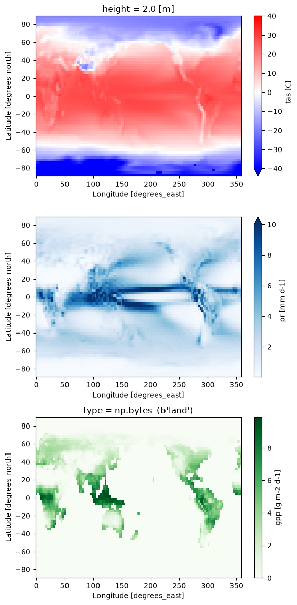

Summary¶

intake-esgf becomes the way that you download or locate data as well as load it into memory. It is a full specification of what your analysis is about and makes your script portable to other machines or even in use with serverside computing. We are actively developing this codebase. Let us know what other features you would like to see.